Spherical Harmonics and Soft Shadows
Motivation
The rendering equation shows we need to solve the integral equation recursively to render a good image. But solve the integral equation is intractable. A straightforward solution is the Monte-carlo integration. But it still suffers from high computation cost and high variance. If we “relax” the quality a little bit, we can turn to find some approximation algorithms. “Good” basis will help us approximate the equation.
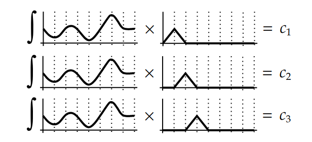
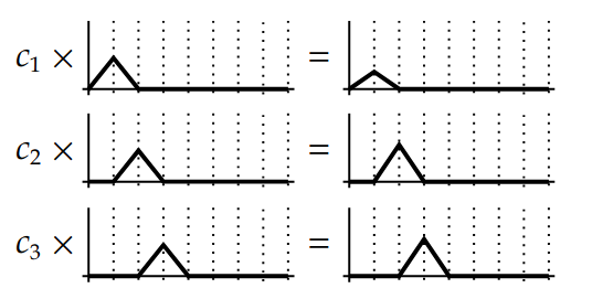
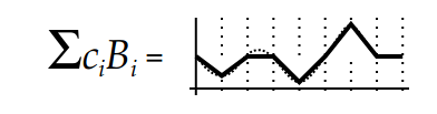
By projecting the function into the basis, we just need to do a dot product to reconstruct the original function. Let’s recap the rendering equation again:
\[L(x, \omega_o) = L_e(x, \omega_o) + \int_S f_r(x, \omega_i, \omega_o) L(x', \omega_i)G(x,x')V(x,x') d\omega_i\]Instead of solving the equation, there is a set of orthonormal basis that approximates the function extremly fast after some precomputation. This magic set of basis is called spherical harmonics (SH).
What is Spherical Harmonics(SH)
Spherical harmonics(SH) are functions defined on the (unit) sphere surface:
\[f(\theta, \phi): R^2 \rightarrow R\]From a high level view, SH defines a set of orthonormal basis functions on the sphere surface. Due to the orthonormal property, it can be a potential tool for basis functions to solve some integrals, e.g. the rendering equations.
To be specific:
\[y_l^m(\theta, \phi) = \begin{cases} \sqrt{2}K_l^m cos(m\phi) P_l^m(cos\theta), m > 0\\ \sqrt{2}K_l^m sin(-m\phi) P_l^{-m}(cos\theta), m < 0\\ K_l^0 P_l^0 cos(\theta), m = 0\\ \end{cases}\] \[K_l^m = \sqrt{\frac{(2l+1)}{4\pi} \frac{(l-|m|)!}{(l+|m|)!}}\] \[l \in \mathbb{R}^+, -l \leq m \leq l\]Here \(P(\cdot)\) is a 1D Legendre polynomials.
\[\begin{align} (l-m)P_l^m &= x(2l-1)P_{l-1}^m - (l+m-1)P_{l-2}^m \\ P_m^m &= (-1)^m (2m-1)!!(1-x^2)^{\frac{m}{2}}\\ P_{m+1}^m &= x(2m+1)P_m^m\\ \end{align}\]Those functions seem to be a little scary for the first time. But the implementation is very simple, see the source.
Another important feature of SH is that it keeps the low frequency details while filtered high frequency details. It is an anology to the fourier transform that maps the spatial domain to frequency domain.
Soft Shadows
As we discussed above, SH can be used to render global illumination effects. Soft shadows are one of the “side product” from global illumination. Soft shadows are the occlusion effects from surrounding objects. The exact value can be be formally defined as:
\[L(x) = \int_S V(x, \omega_i) d\omega_i\]Since SH can help general integral equations, it can also be used for rendering soft shadows. An interesting question is what is the softness of the soft shadow as the order of the SH basis goes higher? Based on this question, I did this experiment.
Experiments
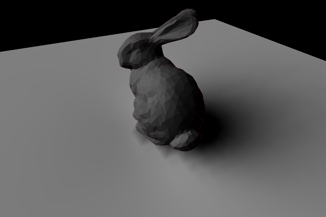
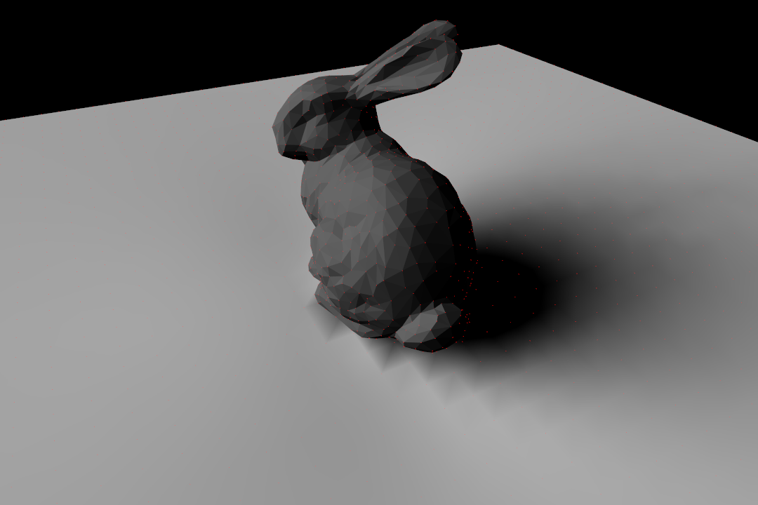
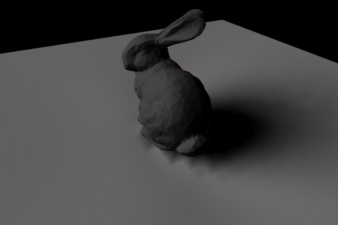
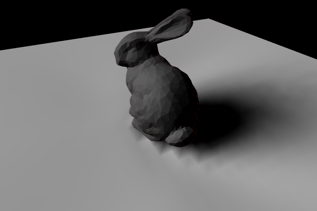
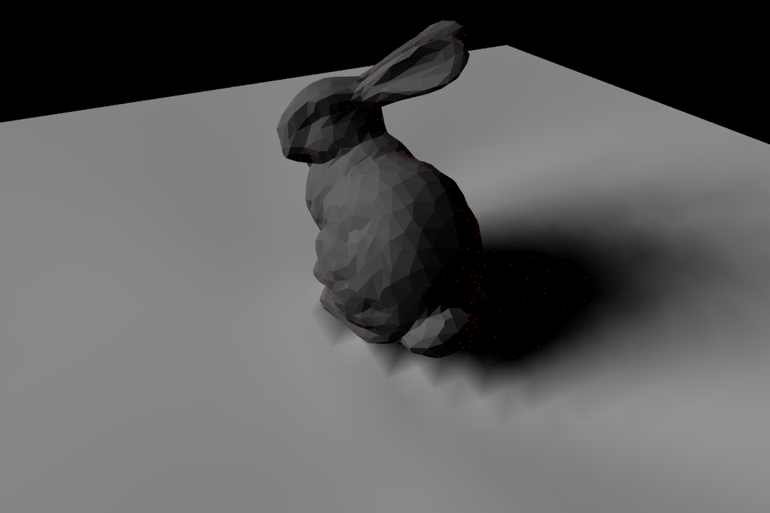
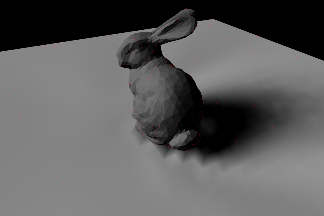
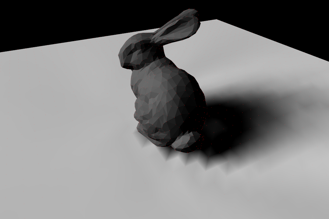
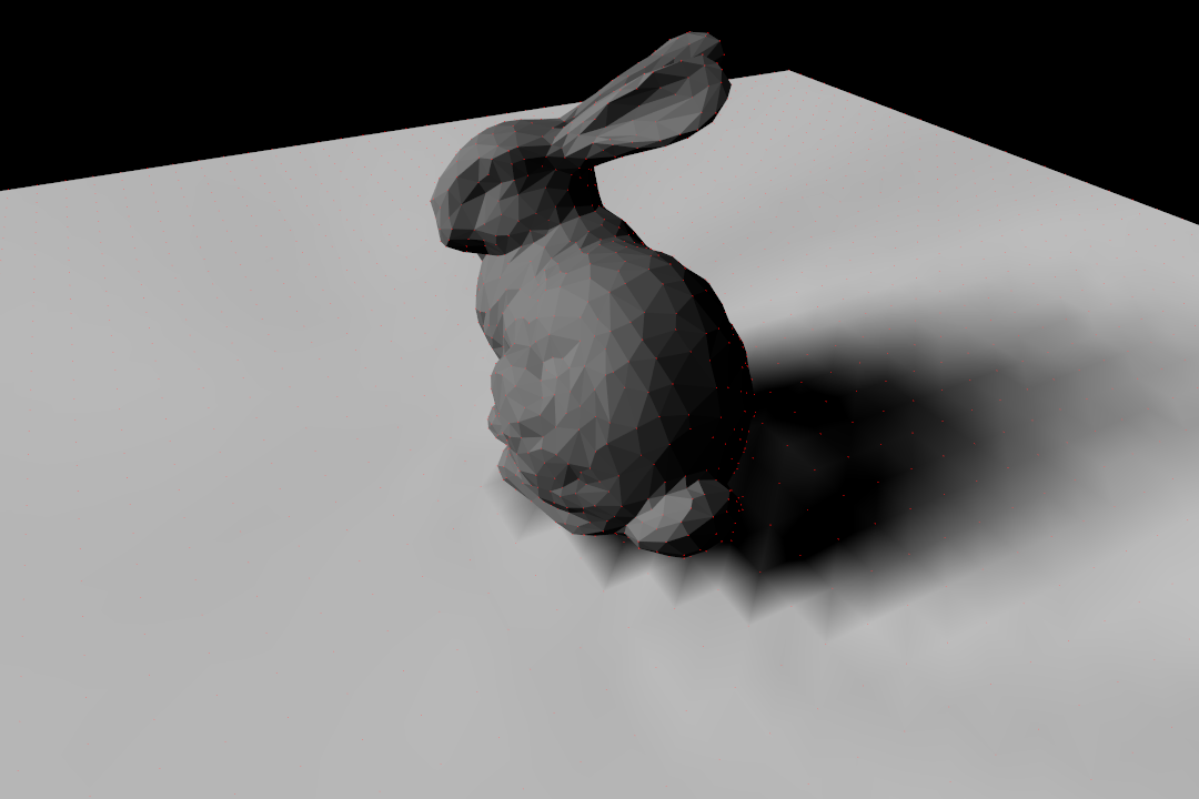
In the scene, I set up a very small area light in the IBL. A bunny is standing on the plane as an occluder for the ground.
|
|
|
|
|
|
|
|
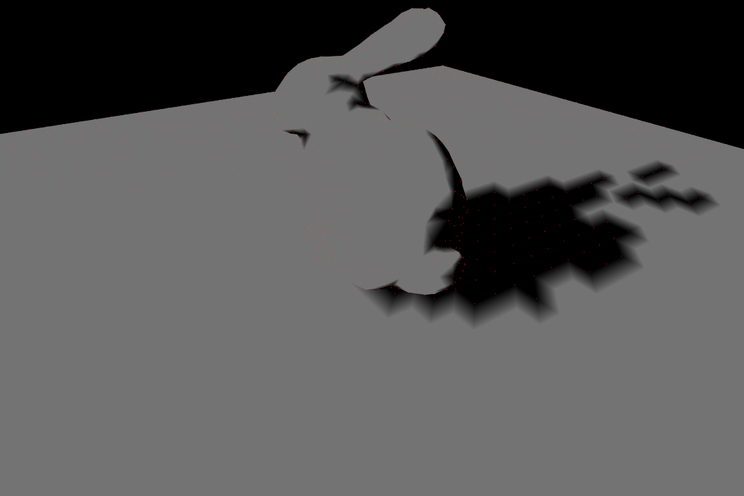
As the order goes higher, the softness is decreasing. But actually for even 11th order(121 bases), the shadow is still a little blurry.
Conclusion
Pros:
- Efficient rendering in runtime
- General basis for integral of spherical surface
- Low frequency details are kept for low orders
Cons:
- Not suitable for hard shadow rendering (of course)
- Shadow resolution may depends on the resolution of the shadow receiver
- For static scene only
It’s not a unexpected results. The experiment seems to be uninteresting. But another problem becomes much more interesting. How to render all frequency shadows using basis approximation? When I did literature review for my paper, I found this paper solved this problem: All-frequency shadows using non-linear wavelet lighting approximation. The basic idea is to use Harr wavelet to compress the environment map and construct a shadow basis matrix, which is very similar to the shadow bases in our paper. It is quite interesting to find the coming ideas solved by others years ago.